Introduction and Disclaimer
This project was born out of a conversation I had with a fellow graduate student at the University of Iowa, Joshua Tschantret, who suggested this data would be cool to have. I was just learning webscraping so I challenged myself to get the data. That challenge led into this becoming a blog post and a component of my portfolio for data science industry applications. As a result, this analysis is preliminary and exploratory. At times it ismore thoroughly descriptive (visually) than anything that would go to publication while also being less than what a final analysis will look like for this project.
Disclaimer: The contents from the forum are displayed in some parts in this blog post. The forum in question is home to white supremacists. The contents of the forum are repugnant, disparaging, and I wholeheartedly do not condone the content of this forum.
Scrape the Data
Generate a Structure for Scraping
The first step in this process is generating a URL for each page of the forum. Each page has 10 posts, and as of the time of starting this project (5/1/2019). The first post’s URL is the website’s base URL followed by the forum ID number. All subsequent pages are numbered with a “-#” before the final forward-slash. I use a simple for loop to generate a vector of all the URLs in the forum. Next, I make an empty dataframe to put the scraped information into. I gather the following:
- Username
- Date
- Time
- Text
#generate a url for each page of the ideology and philosophy forum
ideo_philo_urls <- c("https://www.stormfront.org/forum/t451603/")

#generate a url for each page
for(i in 2:502){
  ideo_philo_urls <- c(ideo_philo_urls, paste0("https://www.stormfront.org/forum/t451603-",
                                               i,
                                               "/"))
}

ideology_forum <- data.frame(user = c(),
                             date = c(),
                             time = c(),
                             text = c())
Loop through the URLs to Scrape the Posts
Now that I have all the URLs of the forum pages in a vector and an empty dataframe to save them in, I execute the following for loop to scrape all of the data from the forum and put it into a dataframe including the variables mentioned above. I scrape the data in 3 parts: the text itself, the date and time together, and then the usernames. The corresponding parts of the webpage scraping are labeled in the code below. I use the stringr package to extract the data that I want.
In the current date of compilation the last forum page does not have a full 10 comments but the comment extraction temporary object still has a length of 10 while the date, time, and user vectors have fewer than 10. To avoid this mistake causing an error and haulting the knit of the document I specify that the loop adds the new posts to the full dataframe for all loops except the last one. I add the last set of posts into the dataframe separately.
for(i in 1:length(ideo_philo_urls)){
  page <- read_html(url(ideo_philo_urls[i]))

#read the text from the posts
  page_text_prelim <- page %>%
    html_nodes("#posts .alt1") %>%
    html_text()

#extract the text from the posts. Every other index in this vector is the post, with the remaining indices being missing.
  page_text <- page_text_prelim[seq(1, 20, 2)]


  page_date_time <- page %>%
    html_nodes("#posts .thead:nth-child(1)") %>%
    html_text()

  page_date_time_prelim <- page_date_time %>%
                           data.frame() %>%
                           janitor::clean_names() %>%
                           mutate(date = stringr::str_extract(x,
                                                              "\\d{2}\\-\\d{2}\\-\\d{4}"),
                                  time = stringr::str_extract(x,
                                                              "\\d{2}\\:\\d{2}\\s[A-Z]{2}")) %>%
                           filter(!is.na(date)) %>%
                           select(date,
                                  time)

  page_date <- as.vector(page_date_time_prelim$date)
  page_time <- as.vector(page_date_time_prelim$time)

  page_user_prelim <- page %>%
                      html_nodes("#posts .alt2") %>%
                      html_text() %>%
                      data.frame() %>%
                      janitor::clean_names() %>%
                      mutate(text = as.character(x),
                             user_time_detect = as.numeric(stringr::str_detect(text,
                                                             "Posts:")),
                             user = stringr::str_extract(text,
                                       "([A-z0-9]+.)+")) %>%
                      filter(user_time_detect == 1) %>%
                      select(user)

  page_user <- as.vector(page_user_prelim$user)

#as of 5/6/2019 this errors on the final loop because the last page only has 7 posts and the page_date and page_time. I have the following if condition to prevent the last loop from erroring.
  if(i < 502){

  page_df <- data.frame(user = as.character(page_user),
                        date = as.character(page_date),
                        time = as.character(page_time),
                        text = as.character(page_text))


  ideology_forum <- rbind(ideology_forum, page_df)
  }
}

#This deals with that last loop that failed

page_text <- as.vector(na.omit(page_text))
page_df <- data.frame(user = as.character(page_user),
                      date = as.character(page_date),
                      time = as.character(page_time),
                      text = as.character(page_text))


ideology_forum <- rbind(ideology_forum, page_df)
Clean the Scraped Data
The code below is cleaning the data captured above. There are several problems with irrelevant text in the posts. The first problem is that each post has the first three word-like objects as “Re: National Socialism” because that is the name of the forum. These three words are not relevant to actually discerning what is being discussed and is therefore removed. The second problem is that many of the posters quote each other and outside materials in their back and forth. In this project I am only interested in novel components of each post. Thus, I remove all quoted text from each post. The third problem is line breaks and other control characters. Fourth, I remove all punctuation from the text for more succinct analysis.
The column “text_nore” is the post itself without the initial indicator that it is a response to the forum. Removing the text in this context is pretty straightforward because I only care about exclusively one phrase that does not appear elsewhere.
The column “text_noquote” is the text of the post remaining from text_nore also minus the text in quotes. This was a rather challenging piece of text to address. There is an example post in its raw form below that shows just how tricky this part was to solve. The selected example has three quotes: the first names the user quoted, and the following two do not. These two quotes have an inconsistent form, and thus make it difficult to capture all possible different quotes with one regex pattern. However, enough things are the same to make it work. First, all quotes start with the word “Quote:”, so I can easily identify the start of a quote. Second, all quotes end with two line breaks “\n\n”. In between those posts there are several words, control characters, and punctuation. In order to capture these patterns I use the greediest (and laziest) approach that works: match 0 or more of a pattern that may or may not exist within a quote until the two line breaks are matched at the end of the quote. This ultimately works on all quote types, and the final regex form can be seen below.
## [1] "\n\n\nRe: National Socialism\n\n\n\nQuote:\n\n\nOriginally Posted by Garak\n\n\nEver heard of copy and paste? I'll bet you could find it before I could. Give me a page number for quicker reference perhaps.\n\nSurely, in the same time it took you to post the question of what the difference between Socialism and National Socialism is, plus these other bickering posts, you could of \"copy and pasted\" all you wanted.\nQuote:\n\nHandouts? What the hell are you talking about. If asking you to clarify your position is a handout in your mind your little movement won't go anywhere.\n\nYou come into my thread with an interest in national socialism, but you don't bother to read the thread at all. Instead, you expect everyone else to compensate your laziness by digging through and finding it themselves for you, when we've already done our fair share of explaining it ourselves.Read the thread.\nI'm not even a National Socialist, and it annoys me that you would threaten to \"not support NS\" if we don't beckon to your will. NSers are our brothers, all the same. Unity makes us powerful, dissent breaks us.\nQuote:\n\nBTW, where are you in ND?\n\nWith how you've been acting, I'm not sure if I want to tell you.I don't want this thread to turn toward further argument unrelated to the topic.\n\n\n"The problem of removing quotes posed another ‘unsolvable’ problem: some posts caused the mutate line for creating “text_noquote” to hang and never finish no matter how long it ran. I isolated 8 posts that were causing this problem via a manual binary sort until I identified the posts causing the problem. The only solution seems to be removing these posts, which is unfortunate. However, I have just over 5000 comments, so it is not THAT big of a deal.
The final two problems are trivial to solve. I remove all control characters into the column “text_nobreak” with the “\c” regex pattern. I remove all punctuation with the “[[:punct:]]” regex pattern. Therefore, the final column created in the code chunk below, text_nopunct, has the cleanest form.
#Create an ID that matches all the post numbers from the forum. This way I can spot check if necessary.
ideology_forum <- ideology_forum %>%
                  mutate(id = seq_along(user))

#These posts caused the stringr functions below to hang and make R crash.
ideology_forum_removed <- ideology_forum[-c(3294, 3481, 3552, 4102, 4308, 4434, 4908, 5015),]

 cleaning <- ideology_forum_removed %>%
             mutate(text_nore = stringr::str_replace_all(text,
                                                         "Re: National Socialism",
                                                         ""),
                    text_noquote = stringr::str_replace_all(text_nore,
                                                            "Quote.(\\n)*.*(\\n)*((.*)|(\\n*))*\\n{2}",
                                                            ""),
                    text_nobreak = stringr::str_replace_all(text_noquote,
                                                            "\\c*",
                                                            ""),
                    text_nopunct = stringr::str_replace_all(text_nobreak,
                                                            "[[:punct:]]*",
                                                            ""),
                    length = str_count(text_nopunct,
                                       "\\w+"))

user_rank <- cleaning %>%
             count(user,
                   name = "n_posts",
                   sort = T) %>%
             mutate(rank = rank(-n_posts,
                                ties.method = 'min'))
Summary Visuals
Post Frequency
This section will provide some visualizations of who is posting, what they are saying, and how much is in their post. The first figure below shows some simple summary information about the top 50 posters. As is obvious from the graph kayden is by far the most frequent poster, followed up by Kaiserreich and John Hawkwood. There is a large discrepency between the top threee themselves, and the top three and the rest of the posters. Each of the top three are separated by about 100 posts, and only 11 users have posted more than 100 times. Another interesting note from this figure is that the top posters are certainly not examples of ‘post frequently, but post little.’ The bars are all shaded with darker shades indicating more words per post (numbers labels the bars are length/10), and each 100+ poster has at least 60 words per post, indicating that they are contributing in some meaningful way to the debate in the forum.

The following figure shows the relationship, or lack thereof, between the number of posts and the length of the posts. Using the full dataset the OLS line has basically no relationship between frequency and length of posts, an OLS coefficient of only 0.008. It seems that for those underneath the threshold of 100 posts the relationship is much stronger and positive, but after subsetting the same plot (not shown here) I find that excluding the top posters does not make the relationship stronger.

The next visualization is a full timeline of the post history on the forum itself and a timeline of the activity of all users with over 100 posts. For the full timeline of the post I group the scraped data by date, and sum a variable that is equal to one for all posts, thus giving me a value for the number of posts per day. I then create a timeline dataframe for all possible days between the first day of activity and the last day of activity. I use this timeline dataframe to left join with the posts-per-day dataframe to make sure that I have values of zero for all variables in days in which there were no posts. This is necessary to assure that I have all days, and am not excluding any because of no posts existing on any given date.
Similarly, in this chunk I also create a dataframe with a user-month unit of analysis for the users with over 100 posts. I follow the same procedure as above, but I ultimately group the data by month in this case instead of date. This is because the full timeline ultimately has a lot of zero-post days when considering all users, so aggregating to monthly intervals is a good way to assure that I still have within-year variation but having fewer zero values. It is also a more aesthetically pleasing and understandable plot.
#Create a user-month dataframe for all users
user_time <- cleaning %>%
             separate(date,
                      into = c('m', 'd', 'y'),
                      sep = '-',
                      remove = F) %>%
             mutate(date = as.Date(ISOdate(y, m, d)),
                    ym = paste0(y, "-", m)) %>%
             group_by(user, ym) %>%
             add_count(user,
                       name = "n_posts") %>%
             summarise(mean_length = mean(length),
                       n_posts = mean(n_posts)) %>%
             arrange(ym) %>%
             ungroup()

#Isolate the users with more than 100 posts
user_100_time <- user_time %>%
              mutate(user = as.character(user)) %>%
              group_by(user) %>%
              mutate(total_posts = sum(n_posts)) %>%
              filter(total_posts >= 100)

#Create a vector long enough to set as a column in the monthly timeline.
top_users <- unique(user_100_time$user)
top_users_1507 <- c()
for(i in 1:137){
  top_users_1507 <- c(top_users_1507, top_users)
}

#Create a posts per day dataframe from scraped data
posts_day <- cleaning %>%
              separate(date,
                      into = c('m', 'd', 'y'),
                      sep = '-',
                      remove = F) %>%
              mutate(date = as.Date(ISOdate(y, m, d)),
                     post = 1) %>%
              group_by(date) %>%
              summarise(mean_length = mean(length),
                        n_posts = sum(post),
                        n_users = n_distinct(user)) %>%
              arrange(date) %>%
              ungroup()

#Create full possible monthly timeline
timeline_monthly <- data.frame(year = 2008:2019) %>%
            uncount(12) %>%
            group_by(year) %>%
            mutate(month = sprintf("%02d", seq_along(year)),
                   ym = paste0(year, "-", month)) %>%
            filter(ym <= "2019-05") %>%
            ungroup() %>%
            select(ym) %>% #137 total months
            uncount(length(top_users)) %>%  #11 top users * 137 possible months = 1507 user-months
            mutate(user = top_users_1507)

#Join the Top User dataframe with the full monthly timeline, and set missings to 0.
user_month <- left_join(timeline_monthly, user_time) %>%
              mutate(n_month = replace_na(n_posts,
                                          0),
                     mean_length = round(replace_na(mean_length,
                                              0),
                                         2),
                     mean_length10 = round(mean_length/10,
                                           2)) %>%
              group_by(user) %>%
              mutate(n_total = sum(n_month)) %>%
              ungroup() %>%
              select(ym,
                     user,
                     n_month,
                     n_total,
                     mean_length10) %>%
              arrange(user,
                      ym,
                      n_total) %>%
              as.tbl()

#Create a full daily timeline
timeline_daily <- data.frame(date = seq.Date(min(posts_day$date),
                                      max(posts_day$date),
                                      "day"))

#Join the full daily timeline with the posts per day dataframe above and set missings to 0.
posts_daily <- left_join(timeline_daily, posts_day) %>%
              separate(date,
                        into = c('y', 'm', 'd'),
                        sep = '-',
                        remove = F) %>%
               mutate(number_posts = ifelse(!is.na(n_posts),
                                       n_posts,
                                       0),
                      number_users = ifelse(!is.na(n_users),
                                            n_users,
                                            0),
                      mean_length10 = ifelse(!is.na(mean_length),
                                             mean_length/10,
                                             0),
                      ym = paste0(y, "-", m) ) %>%
                arrange(date)
The Full Forum Post History plot below is a bar chart of the number of posts per day throughout the history of the forums activity. It is clear that the beginning of the forum is by far the most active. It has the most posts, and the most users per day (represented by darker columns). Another obvious conclusion is that about a year and a half (June 2011 - December 2012) has no activity. This is somewhat curious. It does not seem to line up with anything in the mass media that I can find. My first thought was that perhaps the website was shut down for a while but I can find no evidence backing this up.
Notably, some of the most intense activity on the site is between Barrack Obama’s formal entry into the presidential race and the 2008 presidential election. It is even more curious as a result that the last year and a half of Obama’s first term is empty.

The following scatterplot shows the relationship between the number of words per post, the number of posts per day, and the number of users per day. Generally speaking, the only days with long posts on average have few posts, and the only days with short posts on average are those with many posts, but this relationship is definitively nonlinear. The only days with many users also tend to have shorter but more frequent posts.

Looking at the post history of the top 11 users presents an interesting picture of who dominated the conversation in different contexts over the first 4 years of the data. None of the top posters are active consistently in the last half of the post, so I do not include the last half in this plot.
Kaiserreich, the user who started the forum, was very active originally but did not maintain his activity past the first year. Kayden, the top poster, is pretty consistently active throughout the post with increases in activity periodically but generally showing a smooth trend. Many of the others are very isolated but intense in the frequency of their posts: John Hawkwood and KB Mansfield in particular have a few intense months of posting, but do not post outside of those windows. It seems likely that most of the top posters are top posters not because of their consistent dedication to discussion in the forum, but because of their individual dedication to particular discussion in the forum. Notably, John Hawkwood and Rob Jones peak at the same time at the end of 2008, perhaps the were arguing with each other?

Next, I break down the posts into two different formats for analysis: unigrams (one word phrases) and bigrams (two word phrases). This breaks each post into one observation per word-like-object in the post. A post that is originally one row and has 50 words in it becomes 50 rows, one per word (or two-word pair in the case of bigrams).
The unigram object is created below, and for the making the plot more readable I take only the top 50 most used words. Some words I manually correct for cognates and misspellings so that I do not have multiple observations per word. Many of these phrases also need to be condensed to one-word phrases, such as “National Socialism” or “Mein Kampf.” The unigram framework treats these as two different words, but they certainly represent one concept together.
data("stop_words")
library(SnowballC)

#Clean some important obvious phrases and remove stop words.
unigram <- cleaning %>%
         mutate(text_clean = str_replace_all(text_nopunct,
                                             "[Nn]ational\\s[Ss]ocialism[A-z]*",
                                             "ns") %>%
                             str_replace_all("[Nn]ational\\s[Ss]ocialist[A-z]*",
                                             "ns") %>%
                             str_replace_all("[Aa]dolf(\\s)*[Hh]itler[A-z]*",
                                             "hitler") %>%
                             str_replace_all("[Hh]itlers*",
                                             "hitler") %>%
                             str_replace_all("[A-z]*[Mm]ein(\\s)*[Kk]ampf[A-z]*",
                                             "meinkampf") %>%
                             str_replace_all("[Nn]ationalis[tm]",
                                             "national") %>%
                             str_replace_all("[A-z]*([Tt]hird|3rd)(\\s)*[Rr]eich[A-z]*",
                                             "3rd_reich") %>%
                             str_replace_all("[Nn]azi",
                                             "nazi")) %>%
         unnest_tokens(word,
                       text_clean) %>%
         select(user,
                time,
                date,
                word,
                id) %>%
         anti_join(stop_words)

#Add the word stemmed words.
unigram <- unigram %>%
         mutate(word_stem = wordStem(word),
                word_stem = ifelse(word == 'hitler' | word == 'ns' | word == 'meinkampf',
                                   as.character(word),
                                   word_stem))

#Create a word count dataframe
unigram_count <- unigram %>%
                   count(word, sort = T) %>%
                   mutate(word = reorder(word, n)) %>%
                   mutate(word_stem = wordStem(word),
                          word_stem = ifelse(word == 'hitler' | word == 'ns' | word == 'meinkampf',
                                             word,
                                             word_stem))
The figure below shows the frequency of the 50 most commonly used words. Many of these results are unsurprising, “ns” is the top word, which is what I recoded to mean “national socialism”. This is the name of the forum, so it is expected that it is one of the most commonly used words. The fact that this expectation is met offers at least some confidence that the topic of conversation within the forum remains on topic, rather than digressing into other things. Many of the words leftover have to do with race, such as “race”, “white”, “jewish”, “aryan”, and other similar references. This website is associated strongly with the Ku Klux Klan (KKK) and other far-right white-extremist racist ideologies. Much of the content of this thread is morally reprehensible and vitriolic in its discussion of race. Other common phrases discuss themes of Nazi Germany (e.g. “hitler”, “germany”, “german”), nationalism, war, and politics. Surprisingly, any reference to the word “nazi” itself is not in the top 50 words, but manually searching the data suggests this is because of the many forms this can take, such as “neo-nazi”, “nazism”, and other forms.

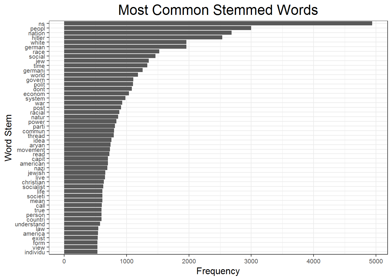
The following figure shows the stemmed unigram counterpart of the unigram chart above. Many of the unigrams are similar, but stemming the words allowed many new words to rise to the top. I stem the words using the SnowballC package. This will reduce words to their etymological stem. Now many words that refer to the same concept have the same stem, and are collapsed into a single bar in the chart. While these word frequency charts are difficult to get much inference from on their own, you can see that stemming the words increases the topic variety of the most used words. Note that “nazi” is now one of the top words but it was not before. The top 50 words are in a table in the appendix with their word stems next to them for curious readers.
#Tidytext does not have the option to remove stop words from sentences, so I use qdap for this.
library('qdap')
data("Top200Words")

#Remove stop words from sentences to make bigrams more meaningful and unnest into bigrams
bigram <- cleaning %>%
         mutate(text_clean = str_replace_all(text_nopunct,
                                             "[Nn]ational\\s[Ss]ocialism[A-z]*",
                                             "ns") %>%
                             str_replace_all("[Nn]ational\\s[Ss]ocialist[A-z]*",
                                             "ns") %>%
                             str_replace_all("[Aa]dolf(\\s)*[Hh]itler[A-z]*",
                                             "hitler") %>%
                             str_replace_all("[Hh]itlers*",
                                             "hitler") %>%
                             str_replace_all("[A-z]*[Mm]ein(\\s)*[Kk]ampf[A-z]*",
                                             "meinkampf") %>%
                             str_replace_all("[Nn]ationalis[tm]",
                                             "national") %>%
                             str_replace_all("[A-z]*([Tt]hird|3rd)(\\s)*[Rr]eich[A-z]*",
                                             "3rd_reich") %>%
                             str_replace_all("[Nn]azi",
                                             "nazi") %>%
                             rm_stopwords(Top200Words,
                                                separate = FALSE)) %>%

         unnest_tokens(bigram,
                       text_clean,
                       token = "ngrams",
                       n = 2) %>%
         select(user,
                time,
                date,
                bigram,
                id)

#Use the tidytext way on the stop-word-removed data using the qdap approach. Similar Results.
bigram_split <- bigram %>%
                separate(bigram, c("word1",
                                   "word2"),
                         sep = " ",
                         remove = F) %>%
                filter(!word1 %in% stop_words$word) %>%
                filter(!word1 %in% stop_words$word) %>%
                filter(!is.na(bigram)) %>%
          count(bigram, sort = T) %>%
          mutate(bigram = reorder(bigram, n))

#Count the frequency of bigrams and order them by frequency.
bigram_sorted <- bigram %>%
          count(bigram, sort = T) %>%
          mutate(bigram = reorder(bigram, n))
The bigram plot below offers a beter view of some of the topics discussed in the forum. The top bigrams are mostly related to Hitler, WWII Germany, nazism, and many forms of discussing National Socialism. They also discuss economic systems and many racial themes. Interestingly, some of the top bigrams are quite violent, such as “fight against” and “war against,” both of which may be advocating war to change current political structures. If one were to read the actual forum it is relatively common that they advocate strong and radical political change through large scale wars as they believe it is the only way national socialism can take hold in the US. By far the most common phrases used have to do with different ways of depicting the white race, examples include: “white race”, “white national(s)”, “white nation,” etc. If these represented one bar, that bar would double the current top phrase of “3rd Reich.”

Sentiment Analysis
# Categorize into Dictionaries
unigram_nrc <- get_sentiments('nrc') %>%
               filter(word != "white") %>% #white is neutral in this context
               inner_join(unigram) %>%
               add_count(sentiment,
                         sort = T) %>%
               inner_join(user_rank)

unigram_nrc_user<- get_sentiments('nrc') %>%
                   filter(word != "white") %>% #white is neutral in this context
                   inner_join(unigram) %>%
                   group_by(user) %>%
                   add_count(sentiment,
                             sort = T) %>%
                   inner_join(user_rank)

# Binary positive or negative
unigram_bing <- inner_join(unigram, get_sentiments("bing")) %>%
                add_count(sentiment,
                          name = "n_sent") %>%
                add_count(sentiment,
                          index = id,
                          name = "n_sent_id") %>%
                add_count(id,
                          name = "num_words") %>%
                inner_join(user_rank)

# -5 to 5 negative to positive
unigram_afinn <- inner_join(unigram, get_sentiments("afinn"))  %>%
                 group_by(id) %>%
                 separate(date,
                          into = c('m', 'd', 'y'),
                          sep = '-',
                          remove = F) %>%
                 mutate(net_score = sum(score),
                        date = as.Date(ISOdate(y, m, d))) %>%
                 select(user,
                        date,
                        id,
                        word,
                        score,
                        net_score) %>%
                 inner_join(user_rank)
The first plot shows the distribution of sentiments from the NRC sentiments dictionary. According to this plot the forum has the most frequency of positive words, followed by negativity, trust, and fear. It is somewhat surprising that positivity dominates this forum is surprising. Negativity, trust, and fear are not surprising. One thing I have not done is control for negation, so I think it is safe to venture that a lot of the trust words are negated, or this group also represents trust themes within the white community, and deep distrust externally. Negativity and fear are at home in a forum like this. Many of the posters hold a real fear that their beloved power structure is threatened, and they are unhappy and scared about this. I am surprised that anger is as low as it is. Of course, keep in mind that this sentiment analysis is only as strong as the dictionaries used, therefore the results are not perfect. You can see top words in each sentiment in the next post.


The plot below shows the distribution of these sentiments between the top users. Overall, these distributions almost all represent exactly the plot above in relative frequency. Positivity, negativity, trust, and fear are the top sentiments among each user, but some users are more emotive than others. This is likely because these are the top posters, such as KB Mansfield, Germania Magna, and kayden.


The following plots uses the “Bing” dictionary in the “tidytext” package to show the percent positive or percent negative within posts across the history of the forum. The first plot shows the posts aggregated by day, and the second plot shows the net postive-negative sentiment per post. Representing the forum by post has two advantages: it shows an alternative way to think of the forum’s flow, and it removes the time gap in the middle to make the plot less elongated. Thinking about the forum in terms of one post following another may be an optimal way to view it. Whoever the most recent poster is, and whenever they are posting, always can see the most recent post even if it was several years ago. The time gap where the forum goes quiet for over a year in the plots above makes the observations of actual posts even harder to see. This plot is still quite difficult to make sense of, but it is better than if there was a large gap from days and months missing.
The net sentiment is the difference between the positive words in a post and the negative words in the post. For the sake of comparison I reduce the positive and negative sentiment of each post to a percentage, with the total number of sentiment-oriented words as the denominator. \(net\,sentiment =\frac{positive\,words}{total\,sentiment\,words} - \frac{negative\,words}{total\,sentiment\,words}\) I only include emotionally charged words in this analysis so that I can determine if a post is mostly negative or mostly postive inasmuch as it is either negative or positive. It would also be reasonable to consider the total non-stop-words as the denominator.
The plots using the Bing dictionary seem to suggest that most days, and indeed most posts, are characterized by being mostly negative, or mostly positive. It also shows that most days are negative than positive, which makes sense coming from such an inherently hateful and dissatisfied forums.

The plot below shows the sentiment anlaysis from the Bing dictionary by post, rather than by day above. Again, most posts are mostly negative or mostly positive, but it looks like the distribution of positive posts and negative posts is about the same, and there are not many strong patterns of negativity or positivity. Somewhere near post 1,000 there is a large chunk of negative posts, but apart from that there are not many distinct patterns of negativity.

The plot below uses the afinn dictionary to do sentiment analysis. This assigns a value to sentiment-oriented words on a -5 to 5 scale, with negative words being negative, and positive words being positive. The first plot shows the net sentiment from the afinn dictionary per day. It is clear that most of the days are more negative than positive, with some days really sticking out above others. One day in June 2009 is the most negative, and one day in December 2009 is the most positive.

This next post is the same as above but using the posts as the unit of analysis rather than each day. The overall sentiment patterns are the same, and not much more is learned here that is not already known from the plots above. However, it served as an important corroboration of previous inferences. On main difference this plot shows is that on average, posts hover around neutral. Nonetheless there are more distinctly negative posts than positive posts.

In sum, the simple sentiment analysis above shows that the posts are much more negative than they are positive. This is not a suprising finding. White supremacists are almost exclusively revisionist individuals, who hold the ideas that whites do not have enough power, and are angry about that. A forum which allows white supremacists to congregate is unsuprisingly very negative in tone.
Latent Dirichlet Allocation
Next I estimate several Latent Dirichlet allocation (LDA) models for each the unigram and the bigram dataframes created and visualized above. LDA models are an unsupervised machine learning tool to identify topics within text based on the frequency with which words appear together and separately. Consider that all bodies of text are made up of topics, and all topics are made up of a particular mixture of words, LDA analysis tries to identify topics based on the distribution of words within and between documents.
I vary the models below by changing the parameter, ‘k.’ This is the number of topics that define the multinomial distribution the LDA model uses while estimating. The larger the k, the more topics the LDA will generate, and thus the more potential nuance uncovered in the discussion. However, in the context of these posts it would be easy to overfit the corpus of text because the posts are all different lengths, some much much longer than others. Smaller posts have less opportunity to discuss any topic than longer posts. In these preliminary analyses I ignore these concerns, but keep them in mind as a secondary step of analysis. I estimate with k values of 2, and 5 with the unigram data, and 2 and 3 with the bigram data.
library(tictoc)

#Two Topic LDA
tic()
unigram_lda2 <- LDA(unigram_dtm,
                    k = 2,
                    control = list(seed = 7117))
toc()
## 28.67 sec elapsed#Five Topic LDA
tic()
unigram_lda5 <- LDA(unigram_dtm,
k = 5,
control = list(seed = 7117))
toc()## 127.67 sec elapsed#Three Topic LDA
tic()
bigram_lda3 <- LDA(bigram_dtm,
k = 3,
control = list(seed = 7117))
toc()## 24.73 sec elapsedThe two topic LDA model is represented visually below. The first plot shows the top 30 unigrams in each topic and their beta value. The beta value is the probability that a word is generated from a topic. NS has about a 0.024% chance of coming from topic 1, but only a 0.005% chance coming from topic 2, as an example. In the context of two topics it seems insufficient to determine what the topics represent. It is noteworthy that the top words of each overlap quite a bit. Overlapping words include: germany, jews, jewish, world, race, ns, political, government, and others. It is plausible that topic one is more referential to the present state of the NS movement, while topic two is more focused on the state of the NS movement during the times of Nazi Germany and WWII. Or, topic two may be more defined by the German experience with NS because some of the top words such as “der” and “die” are German articles, indicating they paired with a German noun and referenced something from Germany. Another possible label for each topic is that topic one could be more associated with the ideological roots of national socialism and discussing those who its primary enemies, while the second topic seems to have more words discussing economic conditions and ideology.

The second plot that compares the beta’s of the two topics illuminates the story of the two topic LDA a little more. The words that are more associated with topic two than topic one are more associated with economics, structure, and community. Words of economic processes, such as demand, production, economy, money, strongly relate to economic themes. Words relating to structure include democracy, systems, nation, country, rights, property, among others. Some of these structure words also relate to community, but most explicit are the words community and children.
Topic one themes seem to focus on Christianity as it relates to nazism, but given the prevalence of meaningless German articles and conjunctions it is difficult to assess the meaning of this group beyond the discussion above. This group does seem to have more discussion in actual German.

The next two plots show the visual results of the LDA analysis with 5 topics. Given the purpose this analysis is primary exploratory without the goal of estimating the absolute best models in this iteration I estimate a 5 topic LDA model just to see what it looks like and how it differs. Surprisingly, the results suggest that there are not very distinct topics within this forum. Perhaps this is unsurprising: white supremacists are the primary users, and the purpose of this particular forum is to discuss national socialism, which has its roots in WWII era Germany. Thus, most topics generated below focus on this time period, and have a slightly different angle on this topic.
The first plot below shows the most popular 30 unigrams by highest beta values per topic. Topic one discusses nationalism socialism with the juxtaposition of words such as white, jewish, and aryan. It is clear that a central theme here is race and heritage, but also religion and the nazi agenda in WWII.
Topic two has a stronger focus on Germany, and uses many words referring to structure, the white race, and nature. It follows that a plausible theme for this topic is the idea that it is natural for the power structure to focus on the white race, and not allocate power outside of the white race.
Topic three seems to have a more general discussion of economic and political systems in America and Germany. It does not have rather specific words discussing power structures, but it does include communism, socialist, and captialism. This indicates that this topic is more focused on economic systems in general, rather than the power structure themes present in the top words in topic two.
Topic four is quite difficult to discern a topic. The only two themes that are represented by multiple words are Jewish people, and Hitler’s 3rd Reich War. Topic five similarly has themes focused on a discussion of the history of Nazi Germany and the violence against Jews.

The plot below is an attempt to show a comparison of beta’s for each word between each topic. With 5 topics, there are 10 (undirected) combinations of each topic. Obviously, juxtaposing the betas for each word of one topic with each word of each other topic cannot be done in one graph. I manually expand the dataframe by ten, and make beta-comparison pairs for all possible combinations. In each pair, I conduct the same comparison as above: log2 of the quotient of the beta from the two comparing topics. In each instance, the larger numbered topic is the numerator, and the smaller numbered topic is the denominator. Topic 5 is always in the numerator, and topic 1 is always in denominator. Also, the titles represent how the models should be interpreted. The subplot titled “Topic 1 - Topic 2” is interpreted as all values less than zero have larger betas, and thus a larger probability of being generated from, topic 1. All values greater than zero belong more to topic 2.
It is my opinion that these plots proove mostly useless in this execution. While the plots above have a reasonable amount of variation between the top words in each plot, comparing the plots produces mostly the same set of words that distinguish each topics. Notably, the years 1932 and 1937, the words: forum, munich, nazism, billion, army, folks, and ns are almost all present in at least one subplot distinguishing one topic from some other topic. So, if these plot suggest the same words distinguish each topic from some other topic, then those words do not effectively distinguish any topics.
Nonetheless, some patterns do exist here. Notably, topic four is distinguished against all others as having primarly Germany words standing out. This is perhaps because of a focus on Germany during WWII. Topic five is starkyl distinguished in these plots as having to do with military topics.
My inference about topic three does not seem to be directly supported here, but neither is it refuted. It seems to have some distinct philosophical components. Topic two and topic one, nonetheless, are not illuminated here.

The plots below show the results of the Bigram LDA analysis. Above I tried two topics and three topics, and I found that two topics showed some difference, but not stronger difference. Five topics showed that it was difficult to discern between groups. As a result, I use a three topic model for bigrams. It is not fair to compare the results here to the results above because there are more bigrams than there are unigrams, and the models are very different because of the difference between one word and two word pairs. I use a three topic model just for exploration using bigrams, and acknowledge that future iterations should test more thoroughly other combinations of topic specifications.
Topic one of the bigram model has a theme focusing on the general future of the white race, especially in ‘competition’ with other races. But discussing phrases like ‘white children,’ ‘future white,’ and ‘war against’ this suggests a focus on the discussion of the future of the white race in general, and violence they believe may be necessary to secure it.
Topic two has a focus on the 20th century life of national socialism, particularly the Nazi party and WWII Germany. This is unsurprising at this point because each topic model has had some topic that has this is at least one of its general themes.
Topic three has a more general focus on the discussion of policy suggestions that may result from national socialism. Many of the phrases that define this topic are different versions of national socialism that aree not captured above as ‘ns’ for some reason, and there is again a theme of economic systems and topics.
The topics uncovered here seem to corroborate some of the findings above: three of the main themes of this forum are the perceived white conflict with other races because of the perceived threats non-whites pose, a discussion of national socialism in the WWII Germany context, and a discussion of the economic (and to a lesser extent political) systems the are prescribed by or threaten national socialism.

The plots below again compare the betas of each topic with all other topics. They follow the convention used above, with the smaller number topic always being the denominator. These plots, similar to the five topic model, do not offer much in the way of corroborating the inferences I made in interpreting the highest betas of each topic.
Topic one here is in some ways defined strongly by a discussion of past racial struggles. But many of the phrases here do not point to a strong thematic overview, other than many of them pointing to discussion of history. Topic two definitely is not illuminated by these plots. These phrases are seemingly unrelated and are definitely not related to the topic that seem to be represented above. Topic three shares these same shortcomings. Similar to the five topic analysis above, this comparison of beta does not prove helpful.

This prompts a discussion of the role of comparing the betas between topics. It is true that comparing betas by dividing betas and logging the quotient shows which words are more relevant to one topic in comparison to another. But, that does not mean that those words define the topics well. The beta comparison plots above are made from dataframes in which all terms are deleted which do not meet a certain threshold for at least one of the topics. The table below shows this information. Because of the number of topics and the size of the sample, the lower limit needs to change with each model. However, the strategy of removing terms from the beta comparison analysis only removes words if a term does not have a beta for any topic that meets the threshold. This allows a term to be at the minimum threshold for one topic, but well below it for all others. This means that this word is not very descriptive of the topic within which its beta is highest, but its beta is still much, much higher than in the other topics. This is not always useful information.
| Term Type | Topic # | Minimum Beta Threshold | Number of Rows Before Filter | Number of Rows After Filter | Percent Reduced |
|---|---|---|---|---|---|
| Unigram | 2 | .001 | 82,324 | 119 | 99.86% |
| Unigram | 5 | .0001 | 205,810 | 45,730 | 77.78% |
| Bigram | 3 | .00001 | 835,794 | 64,038 | 92.34% |
Note: The unigram two topic model and the bigram three topic model has one observation per pair of topics per term, 10 and 3 respectively.
This example below shows that the term ‘heroic archetype’ is much more descriptive of topic three than topic two or topic one, but not at all descriptive of topic three either.
b_lda3_betacomp %>%
  filter(term ==    "heroic archetype")
## # A tibble: 3 x 8
## term topic1 topic2 topic3 id id2 pair log_ratio
## <chr> <dbl> <dbl> <dbl> <dbl> <dbl> <chr> <dbl>
## 1 heroic archetype 0.0000174 8.85e-88 1.47e-89 2 1 21 -273.
## 2 heroic archetype 0.0000174 8.85e-88 1.47e-89 3 2 32 -5.91
## 3 heroic archetype 0.0000174 8.85e-88 1.47e-89 3 1 31 -279.knitr::kable(unigram_count[1:50,] %>% select(-n))| word | word_stem |
|---|---|
| ns | 41158 |
| people | peopl |
| hitler | 41156 |
| white | white |
| german | german |
| national | nation |
| race | race |
| world | world |
| germany | germani |
| dont | dont |
| time | time |
| government | govern |
| socialism | social |
| system | system |
| war | war |
| political | polit |
| jews | jew |
| nation | nation |
| racial | racial |
| economic | econom |
| thread | thread |
| power | power |
| party | parti |
| jewish | jewish |
| movement | movement |
| life | life |
| aryan | aryan |
| true | true |
| capitalism | capit |
| read | read |
| society | societi |
| jew | jew |
| social | social |
| history | histori |
| im | im |
| means | mean |
| america | america |
| american | american |
| idea | idea |
| post | post |
| socialist | socialist |
| nazi | nazi |
| free | free |
| agree | agre |
| money | monei |
| country | countri |
| real | real |
| understand | understand |
| nature | natur |
| simply | simpli |